gdim estimates graph dimension using cross-validated eigenvalues, via the graph-splitting technique developed in https://arxiv.org/abs/2108.03336. Theoretically, the method works by computing a special type of cross-validated eigenvalue which follows a simple central limit theorem. This allows users to perform hypothesis tests on the rank of the graph.
Installation
You can install gdim from CRAN with:
install.packages("gdim")

# to get the development version from GitHub:
install.packages("pak")
pak::pak("RoheLab/gdim")
Example
eigcv() is the main function in gdim. The single required parameter for the function is the maximum possible dimension, k_max.
In the following example, we generate a random graph from the stochastic block model (SBM) with 1000 nodes and 5 blocks (as such, we would expect the estimated graph dimension to be 5).
library(fastRG)
#> Loading required package: Matrix

B <- matrix(0.1, 5, 5)
diag(B) <- 0.3

model <- sbm(
  n = 1000,
  k = 5,
  B = B,
  expected_degree = 40,
  poisson_edges = FALSE,
  allow_self_loops = FALSE
)

A <- sample_sparse(model)
Here, A is the adjacency matrix.
Now, we call the eigcv() function with k_max=10 to estimate graph dimension.
library(gdim)

eigcv_result <- eigcv(A, k_max = 10)
#> 'as(<dsCMatrix>, "dgCMatrix")' is deprecated.
#> Use 'as(., "generalMatrix")' instead.
#> See help("Deprecated") and help("Matrix-deprecated").
eigcv_result
#> Estimated graph dimension:    5
#>
#> Number of bootstraps:         10
#> Edge splitting probabaility:  0.1
#> Significance level:       0.05
#>
#>  ------------ Summary of Tests ------------
#>   k          z        pvals         padj
#>   1 59.7488180 2.220446e-16 2.220446e-15
#>   2 12.9094629 2.220446e-16 2.220446e-15
#>   3 11.8600427 2.220446e-16 2.220446e-15
#>   4 11.9412340 2.220446e-16 2.220446e-15
#>   5  9.0252520 2.220446e-16 2.220446e-15
#>   6 -0.8512008 8.026711e-01 1.000000e+00
#>   7 -0.8182195 7.933841e-01 1.000000e+00
#>   8 -0.9912649 8.392219e-01 1.000000e+00
#>   9 -0.9005808 8.160944e-01 1.000000e+00
#>  10 -1.1677953 8.785553e-01 1.000000e+00
In this example, eigcv() suggests k=5.
To visualize the result, use plot() which returns a ggplot object. The function displays the test statistic (z score) for each hypothesized graph dimension.
plot(eigcv_result)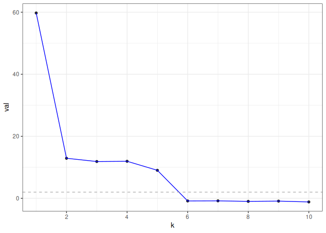
Reference
Chen, Fan, Sebastien Roch, Karl Rohe, and Shuqi Yu. “Estimating Graph Dimension with Cross-Validated Eigenvalues.” ArXiv:2108.03336 [Cs, Math, Stat], August 6, 2021. https://arxiv.org/abs/2108.03336.